単純な2D point-to-point ICP アルゴリズム

Tags:Robotics

2026-09-05

この記事では、単純な2Dのpoint-to-point Iterative Closest Point (ICP)の実装や式の導出について説明します。

point-to-point ICP 1は、2つの点群間の移動距離と回転を求める手法です。 LiDARを積んだロボットに対してICPすることで、ロボットの姿勢を指定することができるようになります。

2つの点群から姿勢を推定する問題

ICPで解きたい問題は、2つの点群間の移動距離と回転の量です。

この図は、点群sourceとそれを(10, 5)分移動し、60度回転したtargetという点群を示しています。

2つの点群の例

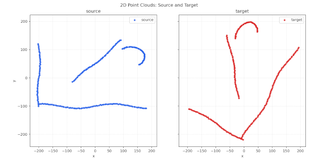
ICPは、このsourceとtargetを入力にとり、移動量である(10, 5)と回転量の60度を出力します。

アルゴリズム

単純には、点群pがqに限りなく同じになるまで回転と平行移動の推論と移動を繰り返します。複数回繰り返す理由は、点群の対応関係を正確に出すことができないからです。

1回のイテレーションは次のような手順で行います。 Orthogonal Procrustes problem 2 3を解きます。

1. 両方の点群の対応関係を求め、対応関係にある点のみ今回のイテレーションの計算に使う
2. 両方の点群の重心を求める
3. 重心が原点にくるように2つの点群を移動する
4. 回転を推定する
5. 移動量を推定する
6. 最初の点に回転と移動を反映する

最後に移動量と回転量の各総和が、2つの点群の移動量と回転量です。

点群の対応関係を求める

片側の点群のある点がもう片方の点群のどの点と対応するか求めます。これは単純に距離(ユークリッド距離)が一番近いものを対応する点とします。

なお、点 $p_{k}$ と点 $p_{k + 1}$ のどちらも点 $q_{l}$ に対応することは問題ありません。

点群の重心を求める

単純に点群の重心は、単に平均座標です。

\overline{p_{x}} = \frac{1}{N} \sum_{i}^{N} p_{i x} \overline{p_{y}} = \frac{1}{N} \sum_{i}^{N} p_{i y}

回転を推定する

2Dの場合は、下の数式のセクションで導出しますが、点の内積和、外積和、atan2で求めます。

def estimate_angle(points, matched, centroid_points , centroid_matched):
    px,py = centroid_points
    qx,qy = centroid_matched

    dot = 0.0
    cross = 0.0
    for p, q in zip(points, matched):
        ax, ay = p[0] - px, p[1] - py
        bx, by = q[0] - qx, q[1] - qy
        dot += ax * bx + ay * by
        cross += ax * by - ay * bx

    return math.atan2(cross, dot)

移動の推定

求めた回転で点群1つめのフレームの重心を回転させたものと 2つめのフレームの重心の差ベクトルが移動量になります。

実装

import math
from typing import Sequence, Tuple

Point = Tuple[float, float]
Pose = Tuple[float, float, float]

def calc_centroid(points):
    return (sum(p[0] for p in points) / len(points),
            sum(p[1] for p in points) / len(points))

def estimate_angle(points, matched, centroid_points , centroid_matched):
    px,py = centroid_points
    qx,qy = centroid_matched

    dot = 0.0
    cross = 0.0
    for p, q in zip(points, matched):
        ax, ay = p[0] - px, p[1] - py
        bx, by = q[0] - qx, q[1] - qy
        dot += ax * bx + ay * by
        cross += ax * by - ay * bx

    return math.atan2(cross, dot)

def estimate_transform(points, matched):
    px,py = calc_centroid(points)
    qx,qy = calc_centroid(matched)

    angle = estimate_angle(points, matched, (px,py), (qx,qy))

    # calc translaction
    c, s = math.cos(angle), math.sin(angle)
    tx = qx - (c * px - s * py)
    ty = qy - (s * px + c * py)
    return tx,  ty, angle

def point_to_point_icp(
    source: Sequence[Point],
    target: Sequence[Point],
    max_iterations: int = 50,
    tolerance: float = 1e-6,
) -> Pose:
    points = [(float(x), float(y)) for x, y in source]
    targets = [(float(x), float(y)) for x, y in target]

    total_angle = 0.0
    total_tx = 0.0
    total_ty = 0.0

    for _ in range(max_iterations):
        matched = [
            min(targets, key=lambda q: (p[0] - q[0]) ** 2 + (p[1] - q[1]) ** 2)
            for p in points
        ]

        tx, ty, angle = estimate_transform(points, matched)

        c, s = math.cos(angle), math.sin(angle)
        # new points
        points = [(c * x - s * y + tx, s * x + c * y + ty) for x, y in points]

        # calc sum of the amount of translation
        total_tx, total_ty = (
            c * total_tx - s * total_ty + tx,
            s * total_tx + c * total_ty + ty,
        )
        total_angle = math.atan2(
            math.sin(total_angle + angle), math.cos(total_angle + angle)
        )

        if math.hypot(tx, ty) < tolerance and abs(angle) < tolerance:
            break

    return total_tx, total_ty, total_angle

推論の途中経過の観察

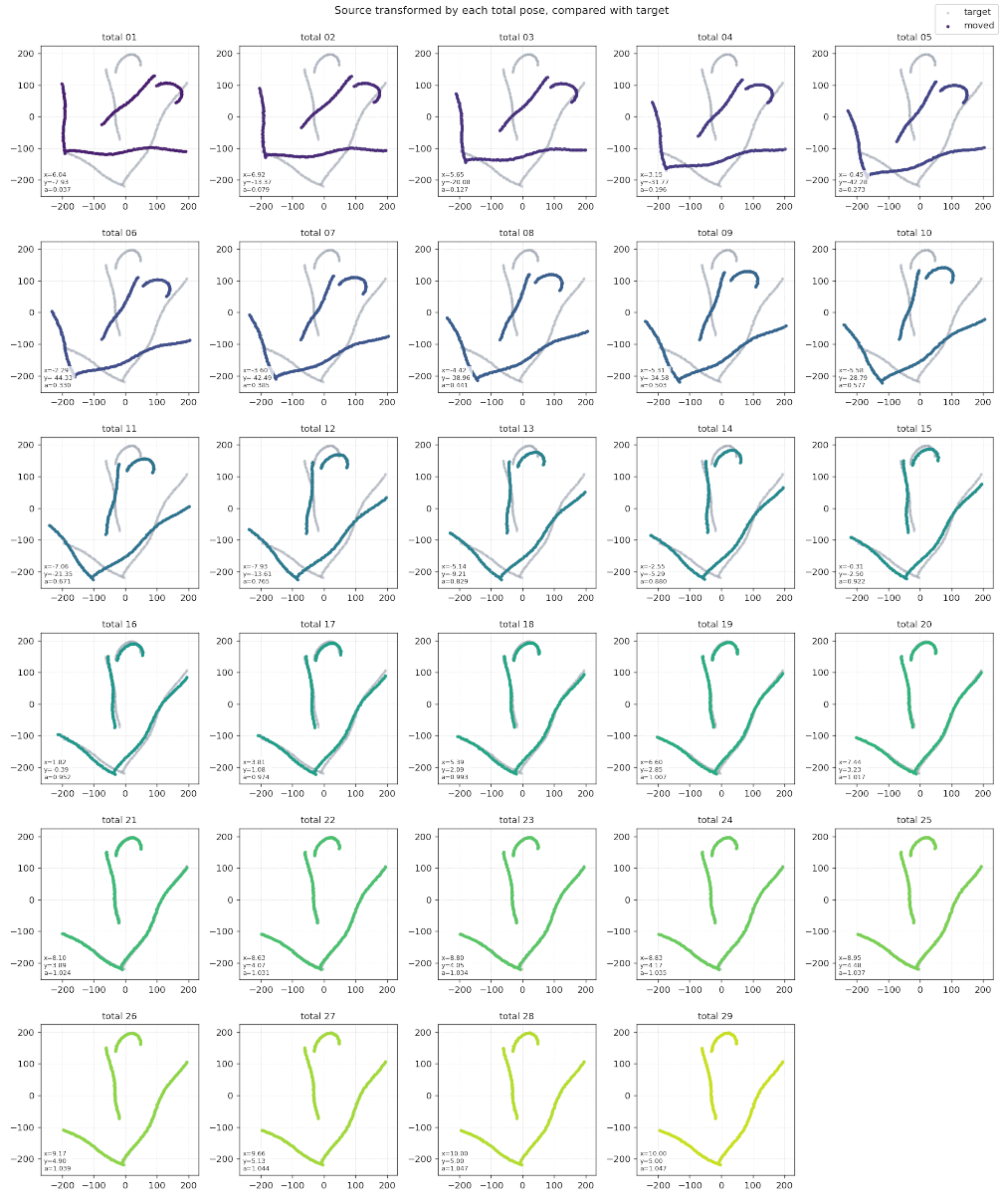
冒頭の例で示した点群を実際にこのプログラムで推論し、その途中状態を表示してみました。グレーの点群が移動後の点群で、色つきのものは各イテレーションで推論した移動を反映したもとの点群です。

iter20ほどで推論がほぼ収束してそうです。

推論の途中経過の観察

角度θを出す式の導出

それぞれ、原点に重心が来るように移動した点群を $p_{i}'$ , $q_{i}'$ とします。

目的関数は次のようになります。ここで、 $R^{⊤} R = I$ を使います。

E (R (θ)) = \sum_{i} {‖ q_{i}' - R (θ) p_{i}' ‖}^{2} = \sum_{i} ({‖ q_{i}' ‖}^{2} + {‖ p_{i}' ‖}^{2} - 2 q_{i}'^{⊤} R (θ) p_{i}')

$R (θ)$ に関係ない部分を除外すると、次のようなargmin問題になります。

a r g m i n \sum_{i} - 2 q_{i}'^{⊤} R (θ) p_{i}'

さらにargminを解くのに係数も不要で、符号を逆転しargmaxにします。

a r g m a x \sum_{i} q_{i}'^{⊤} R (θ) p_{i}'

2Dの回転は1変数なので、微分で角度θをだすことができます。

SVDでθを出す版も書いておきます。

3Dは回転は3軸のため微分ではなく特異値分解(SVD)等で求める必要があります。

微分で角度θを出す

1軸の回転行列は、

R (θ) = (\begin{matrix} c o s (θ) & - s i n (θ) \\ s i n (θ) & c o s (θ) \end{matrix})

$p_{i}'$ と $q_{i}'$ は、

p_{i}' = (\begin{matrix} p_{i x}' \\ p_{i y}' \end{matrix}) q_{i}' = (\begin{matrix} q_{i x}' \\ q_{i y}' \end{matrix})

とします。

$q_{i}'^{⊤} R (θ) p_{i}'$ を展開すると、

q_{i}'^{⊤} R (θ) p_{i}' = (q_{i x}' p_{i x}' + q_{i y}' p_{i y}') c o s (θ) + (q_{i y}' p_{i x}' - q_{i x}' p_{i y}') s i n (θ)

ここで、全ての点についてまとめ、

A = \sum_{i} q_{i x}' p_{i x}' + q_{i y}' p_{i y}' B = \sum_{i} q_{i y}' p_{i x}' - q_{i x}' p_{i y}'

とすると、

a r g m a x f (θ) = A c o s (θ) + B s i n (θ)

を解く問題となります。

微分すると、

\frac{d f}{d θ} = - A s i n (θ) + B c o s (θ)

なので、

- A s i n (θ) + B c o s (θ) = 0

t a n (θ) = \frac{B}{A}

\leftrightarrow θ = a t a n 2 (B, A) = a t a n 2 (\sum_{i} q_{i y}' p_{i x}' - q_{i x}' p_{i y}', \sum_{i} q_{i x}' p_{i x}' + q_{i y}' p_{i y}')

(SVD) 角度θを出す

$q_{i}'^{⊤} R (θ) p_{i}'$ はスカラーなので、trしてもおなじです。

\sum_{i} t r (q_{i}'^{⊤} R (θ) p_{i}')

trの巡回性を使って変形する。

\sum_{i} t r (q_{i}'^{⊤} R (θ) p_{i}') = t r (R (θ) \sum_{i} p_{i}' q_{i}'^{⊤})

ここで、 $H = \sum_{i} p_{i}' q_{i}'^{⊤}$ とすると、 $t r (R (θ) H)$

さらに、HをSVDし、

H = U Σ V^{⊤}

さらに、巡回性を利用し

t r (R (θ) H) = t r (R (θ) U Σ V^{⊤}) = t r (V^{⊤} R (θ) U Σ)

$Σ$ は、対角成分が非負で他が0なので、最大化には $V^{⊤} R (θ) U$ の対角成分以外は0でよい。また、 $V^{⊤} R (θ) U$ は直交行列なので、各要素は1を超えない。

よって、

V^{⊤} R (θ) U = I

これを変形すると、

R (θ) = V U^{⊤}

これに代入して、 $θ$ を出します。

R (θ) = (\begin{matrix} c o s (θ) & - s i n (θ) \\ s i n (θ) & c o s (θ) \end{matrix})

References

[1] Besl PJ, McKay ND (1992) A method for registration of 3-D shapes
- IEEE Trans Pattern Anal Mach Intell 14:239–256.
- https://ieeexplore.ieee.org/document/121791
[2] Arun, K. Somani, Thomas S. Huang, and Steven D. Blostein (1987) Least-squares fitting of two 3-D point sets
- IEEE Transactions on pattern analysis and machine intelligence 5 (1987): 698-700.
- https://ieeexplore.ieee.org/document/4767965
[3] Schönemann, P. H. A generalized solution of the orthogonal procrustes problem.
- Psychometrika 31, 1–10 (1966).
- https://web.stanford.edu/class/cs273/refs/procrustes.pdf

#Author

#Tags

#Recent entries

単純な2D point-to-point ICP アルゴリズム

2つの点群から姿勢を推定する問題

アルゴリズム

点群の対応関係を求める

点群の重心を求める

回転を推定する

移動の推定

実装

推論の途中経過の観察

角度θを出す式の導出

微分で角度θを出す

(SVD) 角度θを出す

References